Determining the uniqueness of oligonucleotide sequences
and an introduction to epigenetics
- 20 minsI’ve been working in the Bioinformatics team at Michael Smith Genome Sciences Center. Most of my contributions center around building web tools, but I had the opportunity to do some more bioinformatic work as well.
First off, a disclaimer: all of the following is extremely simplified and is mostly based off what I’ve learned at work and read over the past few weeks. Nonetheless, this was a lot of fun to put together, and the subject as a whole is pretty cool.
# Epigenetics and DNA Methylation
The plethora of cell types within an organism share a unifying genome. Despite this genetic unity, the various cell types, functions and phenotypes within an individual’s cytome remain widely varied due to vast differences in their gene expression, both quantitatively and qualitatively. These variances are known to be dictated by so-called epigenetic mechanisms, such that individual cell types and developmental states, within an individual organism, have unique epigenomes. Thus, epigenetic mechanisms are crucially relevant in differentiation and development of all cell types, including those which do so in pathological contexts.[1]
In a nutshell, epigenetics is the study of the mechanisms that cause expression variances within an organism’s cells. One such epigenetic mechanism is DNA methylation, the process through which methyl groups are added to cytosine or adenine, with cytosine methylation being the most widespread in mammalian DNA.[2]

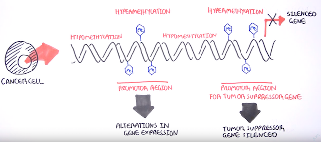
DNA methylation can affect gene expression thanks to how it attracts and repels various DNA-binding proteins due to its position in the DNA helix at what are known as CpG islands. These are often near transcription start sites,[4] and methylation at these sites can cause gene silencing[3] by limiting transcription in the area.

DNA methylation and its gene silencing effects has close associations with the onset of many cancer types[8] - there’s this great video on YouTube by the Garvan Institute of Medical Research that gives a quick rundown of DNA methylation biomarkers and its role in cancers. Epigenetic modifications like hypomethylation (gene activation) and hypermethylation (gene silencing) enable cancer traits such as increased cell growth, immune cell evasion, and the ability to spread to other parts of the other body.
A stronger understanding of how DNA methylation causes cancer has many potential benefits. It can facilitate earlier diagnosis (from easily accessible cancer cells that enter the blood and other bodily fluids) as well as better prediction of how patient might respond to therapy, so as to allow for better treatment recommendations.
There are several methods available to study and analyse DNA methylation. ChIP-seq (the “ChIP” part comes from the role of chromatin immunopercipitation in the process), for example, focuses on examining histone modification.[9]
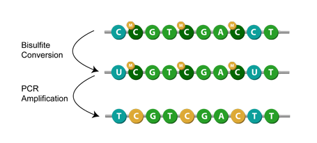
Another method is known as bisulfite conversion, used primarily for studying cytosine methylation. Simply put, it converts unmethylated cytosines to uracils,[1] leaving behind the methylated cytosines. Then, during PCR amplification, the uracil in the bisulfite converted DNA is replaced with thymine.[7] This means that when sequenced, the modification appears as a cytosine to thymine conversion. Given a successful application of bisulfite modification, you can then assume that any remaining cytosines were originally methylated cytosines.[1]
My team often receives such bisulfite converted sequences, albeit with an additional inertesting step: samples are spiked with unmethylated lambda phage, a procedure often done[5][6] to determine the efficiency of the conversion. Due to the lack of methylated cytosine residues in the lambda, if the conversion reaction is complete, all of the lambda sequence’s cytosine should be converted to uracil when aligned to the lambda genome. This conversion rate is used to assess the effectiveness of the bisulfite conversion, which we provide as feedback to the lab or our collaborators.
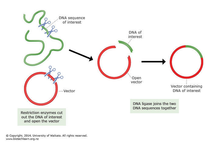
The process of bisulfite conversion has an important consequence: to identify normal samples, we typically use the application of plasmid spike-ins. These are random, known sequences of around 180 base pairs that are grown in a lab, then added to samples during preparation for sequencing. The name “plasmid spike-in” comes from the way the oligonucleotide is incorporated into the pCR-TOPO4 plasmid vector and cloned in E. coli. During quality control, we check for the presence of these spike-ins in our pre-alignment pipelines. If the expected spike-in is only found in very small quantities, then that is usually a red flag that a sample swap might have occurred.
These spike-ins do get affected by the bisulfite conversion, and in the event a perfect or near-perfect conversion, then the reduced complexity of the spike-in sequences (the result of replacing all cytosines with thymines) could potentially cause our pipeline to mistakenly identify spike-ins that aren’t actually there in the sample.
To address these concerns, I was tasked with checking if our plasmid spike-ins are still sufficiently unique following bisulfite conversion, so that the team could decide if we can continue to use the spike-ins as identifiers in bisulfite converted libraries.
# Assessing Oligonucleotide Uniqueness
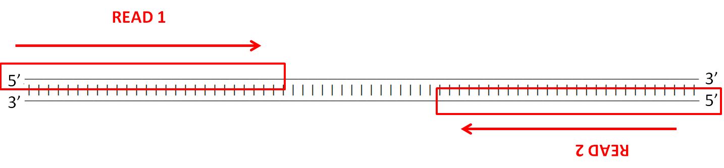
To assess the spike-ins, the reverse complement of each sequence had to be generated, as well as the bisulfite modified versions and their reverse complements. The reverse complement is important to take into consideration due to the way the Illumina’s (the company that builds our sequencers) paired-end sequencing works - strands are sequenced from adapters on both ends.
The details of the sequencing process is a fascinating topic as well, but I’ll leave that for another blog post. Anyway, here’s an example of the different versions of each spike-in that has to be generated:
Original:   AATGTCGATTCGA   ->  Reverse Complement: TCGAATCGACATT
                 |    |
Converted:  AATGTTGATTTGA   ->  Reverse Complement: TCAAATCAACATT
Note that the the original sequence’s reverse complement is not the bisulfite conversion of the original sequence’s bisulfite conversion’s reverse complement (yikes, that was a mouthful). This means that another sequence must be taken into account:
Original RC:   TCGAATCGACATT
                |    |  |
Converted RC:  TTGAATTGATATT
Other than that minor hitch, the conversion was fairly straight forward. I simply created a dictionary for the appropriate conversions and set up a small helper module to do the dirty work:
COMPLEMENT = {
    'a': 't',
    'c': 'g',
    'g': 'c',
    't': 'a'
}
BISULPHITE_CONVERTED = {
    'c': 't'
}

def reverse_complement(seq):
    bases = list(seq.lower())
    bases = [COMPLEMENT.get(base,base) for base in reversed(bases)]
    return ''.join(bases)

def bisulphite_convert(seq):
    bases = list(seq.lower())
    bases = [BISULPHITE_CONVERTED.get(base,base) for base in bases]
    return ''.join(bases)
Now, all these converted sequences are fine and dandy but I needed them in a useful format. This is where the FASTA format and the sprawling Biopython library came in handy.
The FASTA format, unlike the more detailed and usually more practical FASTQ format (which includes quality scores for each nuecleotide!!!), is quite simple: it only has a bit of descriptive metadata and then the sequence itself.
>candidate_2877_original candidate_2877
tatgttgaagtccctagtcgtatggaaagcgttggcatacaagaagcatttcgaacagcc
cttcatcattttagtacaaagttctaatccataactatttcattacaagacccttatagg
catgttacacatttaaatgtcatacgaccgagaaatattttgcatttaaatacctgctaa
gggcgaattcgcccttaattaactgggctcgttgtgcacattgtgttctcttaaaaagtt
Biopython offers a clean, easy way to generate and write these entries to files through its comprehensive SeqIO module:
# ...
record = SeqRecord(
    Seq(bisulphite_seq, None), id='candidate_'+str(c[0])+'_bisulphite_converted'
)
records_converted.append(record) # make a list of all the sequences
# ...
SeqIO.write(records_converted, 'bisulphite_converted_spikeins.fa', 'fasta')
Perfect. With all the sequences prepared in neat FASTA files, I move on to the real problem. In order to check if these spike-ins are usable when bisulfite modified, I have to match them against:
- the human genome (don’t want parts of unconverted sequences to be misidentified as spike-ins)
- bisulfite modified human genome
- the NT database, a database of all sorts of micro-organisms
- bisulfite-converted NT database
- unconverted spike-ins
- other bisulfite-modified spike-ins
One weapon of choice within my team for such tasks is blastall, an old (and outdated, I think - it has long been supersceded by the blast+ programs, but this is what we have, so oh well) program specifically designed for finding regions of similarity within sequences. The name “BLAST” stands for “Basic Local Alignment Search Tool”, which seems reasonably self-explanatory and rolls off the tongue quite nicely.
The program is capable of searching for sequences from a FASTA file (where I have my spike-ins) and searching for similarities against a BLAST database. This meant I had to convert a few things (the spike-in FASTA files, and the human genomes, both of which were also in FASTA files) into this database format.
Python makes executing shell commands programmatically pretty simple, which means I was able to run the BLAST command line tools I needed without much fuss. First off, I had to format the relevant FASTA files into databases:
# see blast formatdb documentation
formatdb_command = 'formatdb -p F -i '
os.system(formatdb_command + my_target_fasta)
Then, I had to set up something to run my blastall commands in parallel. I used the subprocess module for this:
def build_blast_command(query, target, output):
    return blastall_command+' -d '+target+' -i '+query+' -o '+output

outputs = {
    'nt_original':    dir + 'nt_original_report.txt',
    'nt_converted':   dir + 'nt_converted_report.txt',
    'human_original': dir + 'human_original_report.txt',
    'human_ct':       dir + 'human_ct_report.txt',
    'human_ga':       dir + 'human_ga_report.txt',
}
commands = [
    build_blast_command(query, nt_db_original, outputs['nt_original']),
    build_blast_command(query, nt_db_converted, outputs['nt_converted']),
    build_blast_command(query, human_db_original, outputs['human_original']),
    build_blast_command(query, human_db_ct, outputs['human_ct']),
    build_blast_command(query, human_db_ga, outputs['human_ga']),
]
processes = [subprocess.Popen(cmd, shell=True) for cmd in commands]
for p in processes: p.wait()
I recommend just reading the documentation for these tools since they have so many options it makes my head spin. I will mention that the -m 8 parameter specifies that the output should be in blast-tab (tab delimited) format. XML was another option, but I found that the reports ended up being absolutely massive in size, and there were some issues opening it on the puny VM I decided to run these on because I didn’t really want to submit a ticket to have Biopython installed on one of our clusters.
Now, to qualify as a proper “hit” for this task, a match must have an identity of at least 30 base pairs - in other words, it must have an exact match of at least 30 base pairs. This is not really a hard rule, but a general guideline - I later increased the threshold upon consulting with my supervisor, who noted that the presence of adapters used in cloning within the sequence might raise some false positives, since most of the spike-ins will share the same adapters.
Each “hit” looks like this:
Query: candidate_4
       candidate_4_bisulphite_converted
  Hit: gi|3805839|emb|AL031986.1| (99461)
       Arabidopsis thaliana DNA chromosome 4, BAC clone F4B14 (ESSA project)
 HSPs: ----  --------  ---------  ------  ---------------  ---------------------
          #   E-value  Bit score    Span      Query range              Hit range
       ----  --------  ---------  ------  ---------------  ---------------------
          0     0.076      46.09      23           [0:23]            [3937:3960]
A “hit” can have multiple HSPs, or High Scoring Pairs. These HSPs can be parsed for more details, down to which exact base pairs came up as a match:
      Query: candidate_2031_bisulphite candidate_2031_bisulphite_converted
        Hit: gi|190350061|emb|CU856335.2| S.lycopersicum DNA sequence from cl...
Query range: [55:87] (1)
  Hit range: [14413:14445] (1)
Quick stats: evalue 3.3e-07; bitscore 63.93
  Fragments: 1 (32 columns)
     Query - TGTTATTTTTATTTTATTTTTATTTTTGGGTT
             ||||||||||||||||||||||||||||||||
       Hit - TGTTATTTTTATTTTATTTTTATTTTTGGGTT

      Query: candidate_484_rc_bisulphite candidate_484_bisulphite_converted_r...
        Hit: 21 CM000683.1 Homo sapiens chromosome 21, GRCh37 primary referen...
Query range: [109:140] (1)
  Hit range: [39684504:39684535] (1)
Quick stats: evalue 1.1e-07; bitscore 61.95
  Fragments: 1 (31 columns)
     Query - ATATTATTTTTTTTTATTTATTTTATTATTA
             |||||||||||||||||||||||||||||||
       Hit - ATATTATTTTTTTTTATTTATTTTATTATTA
The output contains a wealth of detailed data and as a result the reports can be huge - upwards of several gigabytes. The formmatting is also strange too, with several available and apparently very inconsistent formats. Thankfully, with Biopython, it’s not too hard to extract the information needed determine what qualifies as hits in my case (for flexibility, I added different thresholds to check for):
def detect_hits(result, verbose=False):
    '''
    Helper function for detecting hits according to our criteria.
    Returns a dictionary of lists of high scoring pairs (HSPs).
    '''
    thresholds = {
        'low':    [],
        'medium': [],
        'high':   [],
        'xhigh':  [],
    }
    for hit in result:
        for hsp in hit:
            if hsp.aln_span == hsp.hit_span and hsp.hit_id != hit.query_id:
                if 20 < hsp.aln_span < 30:
                    if verbose:
                        print 'IN RANGE 20~30'
                        print hsp
                        print '\n'
                    thresholds['low'].append(hsp)
                elif 30 < hsp.aln_span < 40:
                    if verbose:
                        print 'IN RANGE 30~40'
                        print hsp
                        print '\n'
                    thresholds['medium'].append(hsp)
                elif 40 < hsp.aln_span < 50:
                    if verbose:
                        print 'IN RANGE 40~50'
                        print hsp
                        print '\n'
                    thresholds['high'].append(hsp)
                elif 50 < hsp.aln_span:
                    if verbose:
                        print 'IN RANGE 50+'
                        print hsp
                        print '\n'
                    thresholds['xhigh'].append(hsp)
    return thresholds

def process_report(report, fmt='blast-tab', verbose=False):
    '''
    Helper function for analysing blast reports. Returns hits that
    meet our criteria and prints the number of hits.
    fmt 'blast-tab' and 'blast-xml' recommended.

    Returns a dictionary of lists of hits.
    '''
    for result in SearchIO.parse(report, fmt):
        hits = detect_hits(result, verbose)
        print str(len(hits['low']))    + ' 20-30bp hits found in ' + report
        print str(len(hits['medium'])) + ' 30-40bp hits found in ' + report
        print str(len(hits['high']))   + ' 40-50bp hits found in ' + report
        print str(len(hits['xhigh']))  + ' 50bp+ hits found in '   + report
        return hits
Again, with the help of Biopython, parsing the blast-tab output from the various blastall commands was a piece of cake:
# Parse outputs.
low_threshold = []
med_threshold = []
high_threshold = []
xhigh_threshold = []
print 'Parsing ' + str(outputs.values())
for report in outputs.values():
    hits = process_report(report, verbose=verbose)
    low_threshold   += hits['low']
    med_threshold   += hits['medium']
    high_threshold  += hits['high']
    xhigh_threshold += hits['xhigh']

# Output results.
print '>> Range 20~30bp: ' + str(len(low_threshold))  + ' hits.'
if verbose:
    print [ hit.hit_id+':'+hit.query_id for hit in low_threshold ]
print '>> Range 30~40bp: ' + str(len(med_threshold))  + ' hits.'
if verbose:
    print [ hit.hit_id+':'+hit.query_id for hit in med_threshold ]
print '>> Range 40~50bp: ' + str(len(high_threshold)) + ' hits.'
if verbose:
    print [ hit.hit_id+':'+hit.query_id for hit in high_threshold ]
print '>> Range 50bp+: '   + str(len(xhigh_threshold)) + ' hits.'
if verbose:
    print [ hit.hit_id+':'+hit.query_id for hit in xhigh_threshold ]
And that was more or less it. This particular tool — which I wrapped up as an argparse command line application with a wealth of options — ended up seeing quite a big of use as a handy utility for investigating contamination and sample swap events, and I suppose that’s pretty nice.
I’ll wrap up this post with a bit of trivia: the first human genome took over 12 years and about $1 billion to sequence. Today, with over a decade’s worth of algorithmic and technological advancements, we can now sequence a human genome for a few thousand dollars, in less than a day. Amazing stuff.
# References
[1] O’Sullivan, Eileen, and Michael Goggins. “DNA Methylation Analysis in Human Cancer.” Methods in molecular biology (Clifton, N.J.) 980 (2013): 131–156. PMC. Web. 4 Feb. 2018.
[2] Wu, Tao P. et al. “DNA Methylation on N6-Adenine in Mammalian Embryonic Stem Cells.” Nature 532.7599 (2016): 329–333. PMC. Web. 5 Feb. 2018.
[3] Li, En, and Yi Zhang. “DNA Methylation in Mammals.” Cold Spring Harbour Perspectives in Biology 6.5 (2014): a019133. PMC. Web. 5 Feb. 2018.
[4] Watt, F, and P L Molloy. “Cytosine methylation prevents binding to DNA of a HeLa cell transcription factor required for optimal expression of the adenovirus major late promoter.” Genes & Development, vol. 2, no. 9, Jan. 1988
[5] Ondov, Brian D. et al. “An Alignment Algorithm for Bisulfite Sequencing Using the Applied Biosystems SOLiD System.” Bioinformatics 26.15 (2010): 1901–1902. PMC. Web. 5 Feb. 2018.
[6] Toh, Hidehiro et al. “Software Updates in the Illumina HiSeq Platform Affect Whole-Genome Bisulfite Sequencing.” BMC Genomics 18 (2017): 31. PMC. Web. 5 Feb. 2018.
[7] Wang, R Y, C W Gehrke, and M Ehrlich. “Comparison of Bisulfite Modification of 5-Methyldeoxycytidine and Deoxycytidine Residues.” Nucleic Acids Research 8.20 (1980): 4777–4790. Print.
[8] Ehrich M, Turner J, Gibbs P, Lipton L, Giovanneti M, Cantor C, van den Boom D “Cytosine methylation profiling of cancer cell lines.” Proc Natl Acad Sci USA 105 (2008): 4844–4849
[9] O’Geen, Henriette, Lorigail Echipare, and Peggy J. Farnham. “Using ChIP-Seq Technology to Generate High-Resolution Profiles of Histone Modifications.” Methods in molecular biology (Clifton, N.J.) 791 (2011): 265–286. PMC. Web. 8 Feb. 2018.
# Random
It’s been raining a lot. When it stops raining and the sun comes out, it can be pretty confusing, like that brief feeling you have when you wake up on your friend’s couch after a long night and wonder how you ended up there.

Rain, coffee, cough hee, and rain.
Not to say that “how did I get here?” is a particularly bad question. In fact, it is an excellent question. Here are some other decent (I think) questions I found myself asking recently:
- why would you keep a scary doll, complete with a mini wooden seat, in your guest bedroom?
- why is tumblr’s gif file size limit so damn small?
- where did I leave my bag of rice?
- why is there a wooden giraffe here?
- why does water come out of both of these shower faucets simultaneously?
- what do you do with long hairs that you lose in the shower?
The last question there has, I’ve learned, an ingenious solution: stick it on the shower wall for the next person to admire. The wooden giraffe turned out to be a failed endeavour in setting up a wooden giraffe smuggling business - seems like demand for wooden giraffes was not quite as high as expected.
The rest of the questions were a bit more mysterious and, like most questions, went largely unanswered.